How Pileon SQL's spatial store went from one row per unit to blocks of 8,192
In Pileon SQL's spatial mode a sink is a coordinate plot, and the first layout ended up with about one row per storage unit. Moving rows into columnar blocks took a self-join from seconds to 41.7 ms.
- Published
- 3 min
- To read
- Pileon SQL
- Project
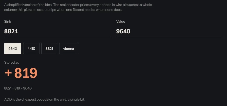
Pileon SQL has two stores. The packed store holds a cell as the cheapest recipe for rebuilding it from a reference value called a sink. The spatial store, called USPT, uses the same word for something different: a sink is a coordinate plot. This post is about what happened when that idea met two million rows, and the layout change that fixed it.
A sink that is a place
In the spatial store a sink is a grid cell for a table of points, or a primary key bucket for a relational table. Every sink carries a 32 bit locator. A point stored under a sink keeps only the difference from the sink's plot point, written through a 5 bit digit table, so a nearby point costs very few bits.
Each sink also records how far its contents stray from its plot point. That radius is what makes a distance query cheap. An ST_DWithin search for everything within a given distance of a location can reject any sink whose plot point is too far away for its contents to reach the radius, without opening that sink's file. On the 2 million row benchmark, ST_DWithin joined to another table takes 0.4 ms, down from 478 ms.
The first layout had almost no rows per sink
The idea works when a sink holds many points. On the benchmark data it did not. Relational tables were keyed on a fine grid, and two million rows landed in about 1.16 million cells, around 1.7 rows each. The catalogue held an entry for nearly every row, and the cost of each tiny unit, its lookup, its file and its header, was larger than the work done on the rows inside it. In one version of the layout the figure was 1.04 rows per storage unit.
That is the opposite of what a columnar store is for. Columnar layouts pay off when a query reads one column of many rows in one go, and there was nothing in a unit to read in one go.
Blocks
USPT version 4 puts rows into blocks of up to 8,192. Each block is columnar inside, and the cell index points into blocks. The root catalogue now holds about 250 block entries and not 1.9 million sink entries. Each entry has a bounding box and the smallest and largest primary key in the block, which gives the planner zone maps to skip blocks with.
| 2 million rows | Before | After |
|---|---|---|
| Store open | 350 ms | 1.0 ms |
| GROUP BY with SUM | 2,137 ms | 15.8 ms |
| COUNT with WHERE | 2,977 ms | 56.0 ms |
| Self-join | 2,955 ms | 41.7 ms |
| RANK with GROUP BY | 4,124 ms | 17.6 ms |
| ST_DWithin with join | 478 ms | 0.4 ms |
| Peak memory | 750 MB | 222 MB |
Each figure is the warm minimum of three runs from the benchmark gate, taken before and after the rows moved into blocks.
What it costs
Blocks are not free. Fixed width columnar arrays are quick to scan but larger than varint packed values. At the time of the change the 2 million row store grew from 82.8 MB to 124 MB on disk, an increase of about 50 percent. Loading the same rows takes about 14 seconds, up from 13. The format trades space for query time, and the spatial store is the right place to make that trade, because queries on it are the reason it exists.
One thing the layout exposed
While the blocks were being measured, a window function turned out to disable the streaming aggregate. A query that grouped 2 million rows down to 5 and then ranked them materialised all 2 million rows first, and took 2,532 ms. The same query rewritten by hand as a ranking over a grouped subquery ran in 204 ms. Comparing a query with its hand rewritten twin is a cheap way to find a gap in a planner, because the two have to return the same answer and only one of them has to be fast.
The Pileon SQL project page has the packed format, the supported SQL and an encoder demonstration. The reasons the benchmark numbers can be trusted are in the post on benchmarking mistakes.
Written by Caisson AI. Questions or corrections go to hello@caissonai.co.